去噪扩散概率模型
作者: A_K_Nain
创建日期: 2022/11/30
最后修改: 2022/12/07
描述: 使用去噪扩散概率模型生成花朵图像。

介绍
生成模型在过去五年经历了巨大的增长。像 VAEs、GANs 和基于流的模型在生成高质量内容,尤其是图像方面取得了巨大的成功。扩散模型是一种新的生成模型,已被证明优于之前的方法。
扩散模型受到非平衡热力学的启发,通过去噪来学习生成。通过去噪学习包括两个过程,每个过程都是马尔可夫链。这些是:
-
正向过程:在正向过程中,我们在一系列时间步骤
(t1, t2, ..., tn)中逐渐向数据添加随机噪声。当前时间步的样本来自高斯分布,分布的均值依赖于前一个时间步的样本,分布的方差遵循固定的计划。在正向过程结束时,样本最终具有纯噪声分布。 -
反向过程:在反向过程中,我们尝试在每个时间步撤销添加的噪声。我们从纯噪声分布(正向过程的最后一步)开始,尝试按照向后方向
(tn, tn-1, ..., t1)对样本去噪。
我们在这个代码示例中实现了 去噪扩散概率模型 的论文,简称 DDPM。它是第一篇证明使用扩散模型生成高质量图像的论文。作者证明了扩散模型的某种参数化在训练过程中与多噪声水平的去噪得分匹配揭示了等价性,以及在采样过程中通过退火的朗之万动力学生成最佳质量结果。
这篇论文复制了涉及扩散过程的两个马尔可夫链(正向过程和反向过程),但针对图像。正向过程是固定的,并根据论文中标记为 beta 的固定方差计划逐渐向图像添加高斯噪声。这是扩散过程在图像中的样子:(图像 -> 噪声::噪声 -> 图像)
论文描述了两个算法,一个用于训练模型,另一个用于从训练模型中采样。训练通过优化负对数似然的通常变分界限进行。目标函数进一步简化,网络被视为噪声预测网络。一旦优化,我们就可以从网络中采样以从噪声样本生成新图像。以下是论文中介绍的两个算法的概述:

注意: DDPM 只是实现扩散模型的一种方式。此外,DDPM 中的采样算法复制了完整的马尔可夫链。因此,与其他生成模型(如 GANs)相比,它在生成新样本方面速度较慢。很多研究努力已致力于解决这个问题。其中一个例子是去噪扩散隐式模型,简称 DDIM,作者用非马尔可夫过程替换了马尔可夫链,以更快地进行采样。您可以在 这里 找到 DDIM 的代码示例。
实现 DDPM 模型很简单。我们定义一个模型,接受两个输入:图像和随机采样的时间步骤。在每个训练步骤中,我们执行以下操作来训练我们的模型:
- 随机采样噪声以添加到输入中。
- 应用正向过程,用采样的噪声扩散输入。
- 您的模型接受这些噪声样本作为输入,并输出每个时间步骤的噪声预测。
- 给定真实噪声和预测噪声,我们计算损失值。
- 然后我们计算梯度并更新模型权重。
考虑到我们的模型知道如何在给定时间步骤去噪噪声样本,我们可以利用这个想法从纯噪声分布开始生成新样本。
设置
import math
import numpy as np
import matplotlib.pyplot as plt

# 需要 TensorFlow >=2.11 以用于 GroupNormalization 层。
import tensorflow as tf
from tensorflow import keras
from tensorflow.keras import layers
import tensorflow_datasets as tfds
超参数
batch_size = 32
num_epochs = 1  # 仅为了演示
total_timesteps = 1000
norm_groups = 8  # 在GroupNormalization层中使用的组数
learning_rate = 2e-4

img_size = 64
img_channels = 3
clip_min = -1.0
clip_max = 1.0

first_conv_channels = 64
channel_multiplier = [1, 2, 4, 8]
widths = [first_conv_channels * mult for mult in channel_multiplier]
has_attention = [False, False, True, True]
num_res_blocks = 2  # 残差块的数量

dataset_name = "oxford_flowers102"
splits = ["train"]
数据集
我们使用 Oxford Flowers 102 数据集来生成花朵的图像。在预处理方面,我们使用中心裁剪将图像调整为所需的图像大小,并将像素值缩放到 [-1.0, 1.0] 范围内。这与 DDPMs 论文 作者所应用的像素值范围一致。为了增强训练数据,我们随机左右翻转图像。
# 加载数据集
(ds,) = tfds.load(dataset_name, split=splits, with_info=False, shuffle_files=True)


def augment(img):
    """随机左右翻转图像。"""
    return tf.image.random_flip_left_right(img)


def resize_and_rescale(img, size):
    """首先将图像调整为所需的大小,然后
    将像素值缩放到 [-1.0, 1.0] 范围内。

    参数:
        img: 图像张量
        size: 调整大小所需的图像尺寸
    返回:
        调整大小并重新缩放的图像张量
    """

    height = tf.shape(img)[0]
    width = tf.shape(img)[1]
    crop_size = tf.minimum(height, width)

    img = tf.image.crop_to_bounding_box(
        img,
        (height - crop_size) // 2,
        (width - crop_size) // 2,
        crop_size,
        crop_size,
    )

    # 调整大小
    img = tf.cast(img, dtype=tf.float32)
    img = tf.image.resize(img, size=size, antialias=True)

    # 重新缩放像素值
    img = img / 127.5 - 1.0
    img = tf.clip_by_value(img, clip_min, clip_max)
    return img


def train_preprocessing(x):
    img = x["image"]
    img = resize_and_rescale(img, size=(img_size, img_size))
    img = augment(img)
    return img


train_ds = (
    ds.map(train_preprocessing, num_parallel_calls=tf.data.AUTOTUNE)
    .batch(batch_size, drop_remainder=True)
    .shuffle(batch_size * 2)
    .prefetch(tf.data.AUTOTUNE)
)
高斯扩散工具
我们将正向过程和反向过程定义为一个单独的工具。这个工具中的大部分代码都借鉴自原始实现,并做了一些小的修改。
class GaussianDiffusion:
    """高斯扩散工具。

    参数:
        beta_start: 计划方差的起始值
        beta_end: 计划方差的结束值
        timesteps: 前向过程中的时间步数
    """

    def __init__(
        self,
        beta_start=1e-4,
        beta_end=0.02,
        timesteps=1000,
        clip_min=-1.0,
        clip_max=1.0,
    ):
        self.beta_start = beta_start
        self.beta_end = beta_end
        self.timesteps = timesteps
        self.clip_min = clip_min
        self.clip_max = clip_max

        # 定义线性方差调度
        self.betas = betas = np.linspace(
            beta_start,
            beta_end,
            timesteps,
            dtype=np.float64,  # 使用 float64 以获得更好的精度
        )
        self.num_timesteps = int(timesteps)

        alphas = 1.0 - betas
        alphas_cumprod = np.cumprod(alphas, axis=0)
        alphas_cumprod_prev = np.append(1.0, alphas_cumprod[:-1])

        self.betas = tf.constant(betas, dtype=tf.float32)
        self.alphas_cumprod = tf.constant(alphas_cumprod, dtype=tf.float32)
        self.alphas_cumprod_prev = tf.constant(alphas_cumprod_prev, dtype=tf.float32)

        # 扩散 q(x_t | x_{t-1}) 和其他计算
        self.sqrt_alphas_cumprod = tf.constant(
            np.sqrt(alphas_cumprod), dtype=tf.float32
        )

        self.sqrt_one_minus_alphas_cumprod = tf.constant(
            np.sqrt(1.0 - alphas_cumprod), dtype=tf.float32
        )

        self.log_one_minus_alphas_cumprod = tf.constant(
            np.log(1.0 - alphas_cumprod), dtype=tf.float32
        )

        self.sqrt_recip_alphas_cumprod = tf.constant(
            np.sqrt(1.0 / alphas_cumprod), dtype=tf.float32
        )
        self.sqrt_recipm1_alphas_cumprod = tf.constant(
            np.sqrt(1.0 / alphas_cumprod - 1), dtype=tf.float32
        )

        # 后验 q(x_{t-1} | x_t, x_0) 的计算
        posterior_variance = (
            betas * (1.0 - alphas_cumprod_prev) / (1.0 - alphas_cumprod)
        )
        self.posterior_variance = tf.constant(posterior_variance, dtype=tf.float32)

        # 由于扩散链开始时后验方差为 0,因此日志计算被截断
        self.posterior_log_variance_clipped = tf.constant(
            np.log(np.maximum(posterior_variance, 1e-20)), dtype=tf.float32
        )

        self.posterior_mean_coef1 = tf.constant(
            betas * np.sqrt(alphas_cumprod_prev) / (1.0 - alphas_cumprod),
            dtype=tf.float32,
        )

        self.posterior_mean_coef2 = tf.constant(
            (1.0 - alphas_cumprod_prev) * np.sqrt(alphas) / (1.0 - alphas_cumprod),
            dtype=tf.float32,
        )

    def _extract(self, a, t, x_shape):
        """在指定的时间步提取一些系数,
        然后重塑为 [batch_size, 1, 1, 1, 1, ...] 以便于广播。

        参数:
            a: 要从中提取的张量
            t: 要提取系数的时间步
            x_shape: 当前批样本的形状
        """
        batch_size = x_shape[0]
        out = tf.gather(a, t)
        return tf.reshape(out, [batch_size, 1, 1, 1])

    def q_mean_variance(self, x_start, t):
        """提取当前时间步的均值和方差。

        参数:
            x_start: 初始样本(在第一次扩散步骤之前)
            t: 当前时间步
        """
        x_start_shape = tf.shape(x_start)
        mean = self._extract(self.sqrt_alphas_cumprod, t, x_start_shape) * x_start
        variance = self._extract(1.0 - self.alphas_cumprod, t, x_start_shape)
        log_variance = self._extract(
            self.log_one_minus_alphas_cumprod, t, x_start_shape
        )
        return mean, variance, log_variance

    def q_sample(self, x_start, t, noise):
        """扩散数据。

        参数:
            x_start: 初始样本(在第一次扩散步骤之前)
            t: 当前时间步
            noise: 在当前时间步要添加的高斯噪声
        返回:
            在时间步 `t` 的扩散样本
        """
        x_start_shape = tf.shape(x_start)
        return (
            self._extract(self.sqrt_alphas_cumprod, t, tf.shape(x_start)) * x_start
            + self._extract(self.sqrt_one_minus_alphas_cumprod, t, x_start_shape)
            * noise
        )

    def predict_start_from_noise(self, x_t, t, noise):
        x_t_shape = tf.shape(x_t)
        return (
            self._extract(self.sqrt_recip_alphas_cumprod, t, x_t_shape) * x_t
            - self._extract(self.sqrt_recipm1_alphas_cumprod, t, x_t_shape) * noise
        )

    def q_posterior(self, x_start, x_t, t):
        """计算扩散的均值和方差
        后验 q(x_{t-1} | x_t, x_0)。

        参数:
            x_start: 后验计算的起点(样本)
            x_t: 在时间步 `t` 的样本
            t: 当前时间步
        返回:
            当前时间步的后验均值和方差
        """

        x_t_shape = tf.shape(x_t)
        posterior_mean = (
            self._extract(self.posterior_mean_coef1, t, x_t_shape) * x_start
            + self._extract(self.posterior_mean_coef2, t, x_t_shape) * x_t
        )
        posterior_variance = self._extract(self.posterior_variance, t, x_t_shape)
        posterior_log_variance_clipped = self._extract(
            self.posterior_log_variance_clipped, t, x_t_shape
        )
        return posterior_mean, posterior_variance, posterior_log_variance_clipped

    def p_mean_variance(self, pred_noise, x, t, clip_denoised=True):
        x_recon = self.predict_start_from_noise(x, t=t, noise=pred_noise)
        if clip_denoised:
            x_recon = tf.clip_by_value(x_recon, self.clip_min, self.clip_max)

        model_mean, posterior_variance, posterior_log_variance = self.q_posterior(
            x_start=x_recon, x_t=x, t=t
        )
        return model_mean, posterior_variance, posterior_log_variance

    def p_sample(self, pred_noise, x, t, clip_denoised=True):
        """从扩散模型中抽样。

        参数:
            pred_noise: 扩散模型预测的噪声
            x: 在给定时间步上预测噪声的样本
            t: 当前时间步
            clip_denoised (bool): 是否将预测的噪声
                限制在指定范围内。
        """
        model_mean, _, model_log_variance = self.p_mean_variance(
            pred_noise, x=x, t=t, clip_denoised=clip_denoised
        )
        noise = tf.random.normal(shape=x.shape, dtype=x.dtype)
        # 当 t == 0 时没有噪声
        nonzero_mask = tf.reshape(
            1 - tf.cast(tf.equal(t, 0), tf.float32), [tf.shape(x)[0], 1, 1, 1]
        )
        return model_mean + nonzero_mask * tf.exp(0.5 * model_log_variance) * noise
网络架构
U-Net,最初是为了语义分割而开发的架构,广泛用于实现扩散模型,但有一些小修改:
- 网络接受两个输入:图像和时间步
- 当我们达到特定分辨率时(论文中为16x16),卷积块之间的自注意力
- 使用组归一化而不是权重归一化
我们实现了大部分原始论文中使用的内容。我们在整个网络中使用swish激活函数。我们使用方差缩放内核初始化器。
这里唯一的区别是GroupNormalization层使用的组数。对于花卉数据集,我们发现groups=8的值相比默认值groups=32能产生更好的结果。Dropout是可选的,并且应在过拟合几率较高的地方使用。在论文中,作者在训练CIFAR10时仅使用了dropout。
# 核心初始化器
def kernel_init(scale):
    scale = max(scale, 1e-10)
    return keras.initializers.VarianceScaling(
        scale, mode="fan_avg", distribution="uniform"
    )


class AttentionBlock(layers.Layer):
    """应用自注意力机制。

    参数:
        units: 密集层的单元数
        groups: 用于GroupNormalization层的组数
    """

    def __init__(self, units, groups=8, **kwargs):
        self.units = units
        self.groups = groups
        super().__init__(**kwargs)

        self.norm = layers.GroupNormalization(groups=groups)
        self.query = layers.Dense(units, kernel_initializer=kernel_init(1.0))
        self.key = layers.Dense(units, kernel_initializer=kernel_init(1.0))
        self.value = layers.Dense(units, kernel_initializer=kernel_init(1.0))
        self.proj = layers.Dense(units, kernel_initializer=kernel_init(0.0))

    def call(self, inputs):
        batch_size = tf.shape(inputs)[0]
        height = tf.shape(inputs)[1]
        width = tf.shape(inputs)[2]
        scale = tf.cast(self.units, tf.float32) ** (-0.5)

        inputs = self.norm(inputs)
        q = self.query(inputs)
        k = self.key(inputs)
        v = self.value(inputs)

        attn_score = tf.einsum("bhwc, bHWc->bhwHW", q, k) * scale
        attn_score = tf.reshape(attn_score, [batch_size, height, width, height * width])

        attn_score = tf.nn.softmax(attn_score, -1)
        attn_score = tf.reshape(attn_score, [batch_size, height, width, height, width])

        proj = tf.einsum("bhwHW,bHWc->bhwc", attn_score, v)
        proj = self.proj(proj)
        return inputs + proj


class TimeEmbedding(layers.Layer):
    def __init__(self, dim, **kwargs):
        super().__init__(**kwargs)
        self.dim = dim
        self.half_dim = dim // 2
        self.emb = math.log(10000) / (self.half_dim - 1)
        self.emb = tf.exp(tf.range(self.half_dim, dtype=tf.float32) * -self.emb)

    def call(self, inputs):
        inputs = tf.cast(inputs, dtype=tf.float32)
        emb = inputs[:, None] * self.emb[None, :]
        emb = tf.concat([tf.sin(emb), tf.cos(emb)], axis=-1)
        return emb


def ResidualBlock(width, groups=8, activation_fn=keras.activations.swish):
    def apply(inputs):
        x, t = inputs
        input_width = x.shape[3]

        if input_width == width:
            residual = x
        else:
            residual = layers.Conv2D(
                width, kernel_size=1, kernel_initializer=kernel_init(1.0)
            )(x)

        temb = activation_fn(t)
        temb = layers.Dense(width, kernel_initializer=kernel_init(1.0))(temb)[
            :, None, None, :
        ]

        x = layers.GroupNormalization(groups=groups)(x)
        x = activation_fn(x)
        x = layers.Conv2D(
            width, kernel_size=3, padding="same", kernel_initializer=kernel_init(1.0)
        )(x)

        x = layers.Add()([x, temb])
        x = layers.GroupNormalization(groups=groups)(x)
        x = activation_fn(x)

        x = layers.Conv2D(
            width, kernel_size=3, padding="same", kernel_initializer=kernel_init(0.0)
        )(x)
        x = layers.Add()([x, residual])
        return x

    return apply


def DownSample(width):
    def apply(x):
        x = layers.Conv2D(
            width,
            kernel_size=3,
            strides=2,
            padding="same",
            kernel_initializer=kernel_init(1.0),
        )(x)
        return x

    return apply


def UpSample(width, interpolation="nearest"):
    def apply(x):
        x = layers.UpSampling2D(size=2, interpolation=interpolation)(x)
        x = layers.Conv2D(
            width, kernel_size=3, padding="same", kernel_initializer=kernel_init(1.0)
        )(x)
        return x

    return apply


def TimeMLP(units, activation_fn=keras.activations.swish):
    def apply(inputs):
        temb = layers.Dense(
            units, activation=activation_fn, kernel_initializer=kernel_init(1.0)
        )(inputs)
        temb = layers.Dense(units, kernel_initializer=kernel_init(1.0))(temb)
        return temb

    return apply


def build_model(
    img_size,
    img_channels,
    widths,
    has_attention,
    num_res_blocks=2,
    norm_groups=8,
    interpolation="nearest",
    activation_fn=keras.activations.swish,
):
    image_input = layers.Input(
        shape=(img_size, img_size, img_channels), name="image_input"
    )
    time_input = keras.Input(shape=(), dtype=tf.int64, name="time_input")

    x = layers.Conv2D(
        first_conv_channels,
        kernel_size=(3, 3),
        padding="same",
        kernel_initializer=kernel_init(1.0),
    )(image_input)

    temb = TimeEmbedding(dim=first_conv_channels * 4)(time_input)
    temb = TimeMLP(units=first_conv_channels * 4, activation_fn=activation_fn)(temb)

    skips = [x]

    # 下采样块
    for i in range(len(widths)):
        for _ in range(num_res_blocks):
            x = ResidualBlock(
                widths[i], groups=norm_groups, activation_fn=activation_fn
            )([x, temb])
            if has_attention[i]:
                x = AttentionBlock(widths[i], groups=norm_groups)(x)
            skips.append(x)

        if widths[i] != widths[-1]:
            x = DownSample(widths[i])(x)
            skips.append(x)

    # 中间块
    x = ResidualBlock(widths[-1], groups=norm_groups, activation_fn=activation_fn)(
        [x, temb]
    )
    x = AttentionBlock(widths[-1], groups=norm_groups)(x)
    x = ResidualBlock(widths[-1], groups=norm_groups, activation_fn=activation_fn)(
        [x, temb]
    )

    # 上采样块
    for i in reversed(range(len(widths))):
        for _ in range(num_res_blocks + 1):
            x = layers.Concatenate(axis=-1)([x, skips.pop()])
            x = ResidualBlock(
                widths[i], groups=norm_groups, activation_fn=activation_fn
            )([x, temb])
            if has_attention[i]:
                x = AttentionBlock(widths[i], groups=norm_groups)(x)

        if i != 0:
            x = UpSample(widths[i], interpolation=interpolation)(x)

    # 结束块
    x = layers.GroupNormalization(groups=norm_groups)(x)
    x = activation_fn(x)
    x = layers.Conv2D(3, (3, 3), padding="same", kernel_initializer=kernel_init(0.0))(x)
    return keras.Model([image_input, time_input], x, name="unet")
训练
我们遵循论文中描述的扩散模型的训练设置。我们使用 Adam 优化器,学习率为 2e-4。我们对模型参数使用 EMA,衰减因子为 0.999。我们将模型视为噪声预测网络,即在每个训练步骤中,我们将一批图像及其相应的时间步骤输入到我们的 UNet 中,网络输出噪声作为预测。
唯一的区别是我们没有使用内核 inception 距离 (KID) 或 Frechet inception 距离 (FID) 来评估训练期间生成样本的质量。这是因为这两种度量标准计算量大,因此为了简洁考虑而被跳过。
注意: 我们使用均方误差作为损失函数,这与论文一致,并在理论上是合理的。然而,在实际运用中,使用均值绝对误差或 Huber 损失作为损失函数也是很常见的。
class DiffusionModel(keras.Model):
    def __init__(self, network, ema_network, timesteps, gdf_util, ema=0.999):
        super().__init__()
        self.network = network
        self.ema_network = ema_network
        self.timesteps = timesteps
        self.gdf_util = gdf_util
        self.ema = ema

    def train_step(self, images):
        # 1. 获取批量大小
        batch_size = tf.shape(images)[0]

        # 2. 统一采样时间步
        t = tf.random.uniform(
            minval=0, maxval=self.timesteps, shape=(batch_size,), dtype=tf.int64
        )

        with tf.GradientTape() as tape:
            # 3. 采样要添加到图像中的随机噪声
            noise = tf.random.normal(shape=tf.shape(images), dtype=images.dtype)

            # 4. 用噪声扩散图像
            images_t = self.gdf_util.q_sample(images, t, noise)

            # 5. 将扩散后的图像和时间步传递给网络
            pred_noise = self.network([images_t, t], training=True)

            # 6. 计算损失
            loss = self.loss(noise, pred_noise)

        # 7. 获取梯度
        gradients = tape.gradient(loss, self.network.trainable_weights)

        # 8. 更新网络的权重
        self.optimizer.apply_gradients(zip(gradients, self.network.trainable_weights))

        # 9. 使用EMA权重更新网络的权重值
        for weight, ema_weight in zip(self.network.weights, self.ema_network.weights):
            ema_weight.assign(self.ema * ema_weight + (1 - self.ema) * weight)

        # 10. 返回损失值
        return {"loss": loss}

    def generate_images(self, num_images=16):
        # 1. 随机采样噪声(反向过程的起点)
        samples = tf.random.normal(
            shape=(num_images, img_size, img_size, img_channels), dtype=tf.float32
        )
        # 2. 从模型中进行迭代采样
        for t in reversed(range(0, self.timesteps)):
            tt = tf.cast(tf.fill(num_images, t), dtype=tf.int64)
            pred_noise = self.ema_network.predict(
                [samples, tt], verbose=0, batch_size=num_images
            )
            samples = self.gdf_util.p_sample(
                pred_noise, samples, tt, clip_denoised=True
            )
        # 3. 返回生成的样本
        return samples

    def plot_images(
        self, epoch=None, logs=None, num_rows=2, num_cols=8, figsize=(12, 5)
    ):
        """使用扩散模型在训练过程中绘制图像的实用工具。"""
        generated_samples = self.generate_images(num_images=num_rows * num_cols)
        generated_samples = (
            tf.clip_by_value(generated_samples * 127.5 + 127.5, 0.0, 255.0)
            .numpy()
            .astype(np.uint8)
        )

        _, ax = plt.subplots(num_rows, num_cols, figsize=figsize)
        for i, image in enumerate(generated_samples):
            if num_rows == 1:
                ax[i].imshow(image)
                ax[i].axis("off")
            else:
                ax[i // num_cols, i % num_cols].imshow(image)
                ax[i // num_cols, i % num_cols].axis("off")

        plt.tight_layout()
        plt.show()


# 构建unet模型
network = build_model(
    img_size=img_size,
    img_channels=img_channels,
    widths=widths,
    has_attention=has_attention,
    num_res_blocks=num_res_blocks,
    norm_groups=norm_groups,
    activation_fn=keras.activations.swish,
)
ema_network = build_model(
    img_size=img_size,
    img_channels=img_channels,
    widths=widths,
    has_attention=has_attention,
    num_res_blocks=num_res_blocks,
    norm_groups=norm_groups,
    activation_fn=keras.activations.swish,
)
ema_network.set_weights(network.get_weights())  # 初始权重相同

# 获取高斯扩散工具的实例
gdf_util = GaussianDiffusion(timesteps=total_timesteps)

# 获取模型
model = DiffusionModel(
    network=network,
    ema_network=ema_network,
    gdf_util=gdf_util,
    timesteps=total_timesteps,
)

# 编译模型
model.compile(
    loss=keras.losses.MeanSquaredError(),
    optimizer=keras.optimizers.Adam(learning_rate=learning_rate),
)

# 训练模型
model.fit(
    train_ds,
    epochs=num_epochs,
    batch_size=batch_size,
    callbacks=[keras.callbacks.LambdaCallback(on_epoch_end=model.plot_images)],
)
31/31 [==============================] - ETA: 0s - loss: 0.7746
31/31 [==============================] - 194s 4s/step - loss: 0.7668

<keras.callbacks.History at 0x7fc9e86ce610>
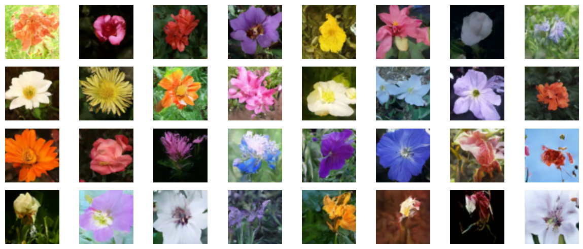
结果
我们在 V100 GPU 上训练了这个模型 800 个周期,每个周期几乎花费 8 秒。我们在这里加载那些权重,并从纯噪声开始生成一些样本。
!curl -LO https://github.com/AakashKumarNain/ddpms/releases/download/v3.0.0/checkpoints.zip
!unzip -qq checkpoints.zip
# 加载模型权重
model.ema_network.load_weights("checkpoints/diffusion_model_checkpoint")

# 生成并绘制一些样本
model.plot_images(num_rows=4, num_cols=8)
  % 总计    % 接收 % 转换  平均速度   时间    时间     时间  当前
                                 下载  上传  总计   花费    剩余  速度
  0     0    0     0    0     0      0      0 --:--:-- --:--:-- --:--:--     0
100  222M  100  222M    0     0  16.0M      0  0:00:13  0:00:13 --:--:-- 14.7M
结论
我们成功地实现并训练了一个扩散模型,完全按照 DDPMs 论文的作者实现的方式。你可以在 这里 找到原始实现。
你可以尝试以下几种方法来改进模型:
-
增加每个块的宽度。更大的模型可以在更少的周期中学习去噪,尽管你可能需要注意过拟合。
-
我们实现了线性调度的方差调度。你可以实现其他方案,如余弦调度,并比较性能。