图像分类与 ConvMixer
作者: Sayak Paul
创建日期: 2021/10/12
最后修改日期: 2021/10/12
描述: 应用于图像块的全卷积网络。

介绍
视觉变换器 (ViT; Dosovitskiy et al.) 从输入图像中提取小块,进行线性投影,然后应用变换器 (Vaswani et al.) 块。将 ViT 应用于图像识别任务正快速成为一个有前途的研究领域,因为 ViT 消除了对强归纳偏置(如卷积)建模局部性的需要。这使得它们成为一种通用计算原语,能够仅从训练数据中学习,同时尽可能减少归纳先验。当使用适当的正则化、数据增强和相对较大数据集进行训练时,ViT 可以获得出色的下游性能。
在论文 Patches Are All You Need 中(注意:在撰写时,这是 ICML 2022 会议的提交),作者扩展了使用图像块训练全卷积网络的思路,并展示了有竞争力的结果。他们的架构名为 ConvMixer,借鉴了最近的各向同性架构,如 ViT、MLP-Mixer (Tolstikhin et al.),例如在网络不同层中使用相同的深度和分辨率、残差连接等。
在这个示例中,我们将实现 ConvMixer 模型,并展示其在 CIFAR-10 数据集上的表现。
导入
import keras
from keras import layers

import matplotlib.pyplot as plt
import tensorflow as tf
import numpy as np
超参数
为了缩短运行时间,我们将仅训练模型 10 个周期。为了专注于 ConvMixer 的核心思想,我们将不使用其他特定于训练的元素,如 RandAugment (Cubuk et al.)。如果您对了解这些细节感兴趣,请参考 原始论文。
learning_rate = 0.001
weight_decay = 0.0001
batch_size = 128
num_epochs = 10
加载 CIFAR-10 数据集
(x_train, y_train), (x_test, y_test) = keras.datasets.cifar10.load_data()
val_split = 0.1

val_indices = int(len(x_train) * val_split)
new_x_train, new_y_train = x_train[val_indices:], y_train[val_indices:]
x_val, y_val = x_train[:val_indices], y_train[:val_indices]

print(f"训练数据样本数: {len(new_x_train)}")
print(f"验证数据样本数: {len(x_val)}")
print(f"测试数据样本数: {len(x_test)}")
训练数据样本数: 45000
验证数据样本数: 5000
测试数据样本数: 10000
准备 tf.data.Dataset 对象
我们的数据增强管道与作者用于 CIFAR-10 数据集的不同,这在示例中是可以的。 请注意,可以将 TF API 用于数据 I/O 和预处理 与其他后端(jax、torch)一起使用,因为在数据预处理方面它是一个功能完备的框架。
image_size = 32
auto = tf.data.AUTOTUNE

augmentation_layers = [
    keras.layers.RandomCrop(image_size, image_size),
    keras.layers.RandomFlip("horizontal"),
]


def augment_images(images):
    for layer in augmentation_layers:
        images = layer(images, training=True)
    return images


def make_datasets(images, labels, is_train=False):
    dataset = tf.data.Dataset.from_tensor_slices((images, labels))
    if is_train:
        dataset = dataset.shuffle(batch_size * 10)
    dataset = dataset.batch(batch_size)
    if is_train:
        dataset = dataset.map(
            lambda x, y: (augment_images(x), y), num_parallel_calls=auto
        )
    return dataset.prefetch(auto)


train_dataset = make_datasets(new_x_train, new_y_train, is_train=True)
val_dataset = make_datasets(x_val, y_val)
test_dataset = make_datasets(x_test, y_test)
ConvMixer 工具
下图(取自原始论文)描绘了 ConvMixer 模型:

ConvMixer 非常类似于 MLP-Mixer,模型之间的主要区别如下:
- 它使用标准卷积层,而不是全连接层。
- 它使用 BatchNorm,而不是典型的 ViT 和 MLP-Mixer 使用的 LayerNorm。 ConvMixer 使用了两种类型的卷积层。(1): 深度卷积,用于混合图像的空间位置,(2): 点卷积(跟随深度卷积后),用于跨补丁混合通道信息。另一个关键点是使用较大的卷积核大小来允许更大的接收场。
def activation_block(x):
    x = layers.Activation("gelu")(x)
    return layers.BatchNormalization()(x)


def conv_stem(x, filters: int, patch_size: int):
    x = layers.Conv2D(filters, kernel_size=patch_size, strides=patch_size)(x)
    return activation_block(x)


def conv_mixer_block(x, filters: int, kernel_size: int):
    # 深度卷积。
    x0 = x
    x = layers.DepthwiseConv2D(kernel_size=kernel_size, padding="same")(x)
    x = layers.Add()([activation_block(x), x0])  # 残差连接。

    # 点卷积。
    x = layers.Conv2D(filters, kernel_size=1)(x)
    x = activation_block(x)

    return x


def get_conv_mixer_256_8(
    image_size=32, filters=256, depth=8, kernel_size=5, patch_size=2, num_classes=10
):
    """ConvMixer-256/8: https://openreview.net/pdf?id=TVHS5Y4dNvM.
    超参数值取自论文。
    """
    inputs = keras.Input((image_size, image_size, 3))
    x = layers.Rescaling(scale=1.0 / 255)(inputs)

    # 提取补丁嵌入。
    x = conv_stem(x, filters, patch_size)

    # ConvMixer 块。
    for _ in range(depth):
        x = conv_mixer_block(x, filters, kernel_size)

    # 分类块。
    x = layers.GlobalAvgPool2D()(x)
    outputs = layers.Dense(num_classes, activation="softmax")(x)

    return keras.Model(inputs, outputs)
本实验中使用的模型称为ConvMixer-256/8,其中 256 表示通道数,8 表示深度。得到的模型只有 0.8 百万参数。
模型训练和评估工具
# 代码参考:
# https://keras.io/examples/vision/image_classification_with_vision_transformer/.


def run_experiment(model):
    optimizer = keras.optimizers.AdamW(
        learning_rate=learning_rate, weight_decay=weight_decay
    )

    model.compile(
        optimizer=optimizer,
        loss="sparse_categorical_crossentropy",
        metrics=["accuracy"],
    )

    checkpoint_filepath = "/tmp/checkpoint.keras"
    checkpoint_callback = keras.callbacks.ModelCheckpoint(
        checkpoint_filepath,
        monitor="val_accuracy",
        save_best_only=True,
        save_weights_only=False,
    )

    history = model.fit(
        train_dataset,
        validation_data=val_dataset,
        epochs=num_epochs,
        callbacks=[checkpoint_callback],
    )

    model.load_weights(checkpoint_filepath)
    _, accuracy = model.evaluate(test_dataset)
    print(f"测试准确率: {round(accuracy * 100, 2)}%")

    return history, model
训练和评估模型
conv_mixer_model = get_conv_mixer_256_8()
history, conv_mixer_model = run_experiment(conv_mixer_model)
Epoch 1/10
 352/352 ━━━━━━━━━━━━━━━━━━━━ 46s 103ms/step - accuracy: 0.4594 - loss: 1.4780 - val_accuracy: 0.1536 - val_loss: 4.0766
Epoch 2/10
 352/352 ━━━━━━━━━━━━━━━━━━━━ 14s 39ms/step - accuracy: 0.6996 - loss: 0.8479 - val_accuracy: 0.7240 - val_loss: 0.7926
Epoch 3/10
 352/352 ━━━━━━━━━━━━━━━━━━━━ 14s 39ms/step - accuracy: 0.7823 - loss: 0.6287 - val_accuracy: 0.7800 - val_loss: 0.6532
Epoch 4/10
 352/352 ━━━━━━━━━━━━━━━━━━━━ 14s 39ms/step - accuracy: 0.8264 - loss: 0.5003 - val_accuracy: 0.8074 - val_loss: 0.5895
Epoch 5/10
 352/352 ━━━━━━━━━━━━━━━━━━━━ 21s 60ms/step - accuracy: 0.8605 - loss: 0.4092 - val_accuracy: 0.7996 - val_loss: 0.6037
Epoch 6/10
 352/352 ━━━━━━━━━━━━━━━━━━━━ 13s 38ms/step - accuracy: 0.8788 - loss: 0.3527 - val_accuracy: 0.8072 - val_loss: 0.6162
Epoch 7/10
 352/352 ━━━━━━━━━━━━━━━━━━━━ 21s 61ms/step - accuracy: 0.8972 - loss: 0.2984 - val_accuracy: 0.8226 - val_loss: 0.5604
Epoch 8/10
 352/352 ━━━━━━━━━━━━━━━━━━━━ 21s 61ms/step - accuracy: 0.9087 - loss: 0.2608 - val_accuracy: 0.8310 - val_loss: 0.5303
Epoch 9/10
 352/352 ━━━━━━━━━━━━━━━━━━━━ 14s 39ms/step - accuracy: 0.9176 - loss: 0.2302 - val_accuracy: 0.8458 - val_loss: 0.5051
Epoch 10/10
 352/352 ━━━━━━━━━━━━━━━━━━━━ 14s 38ms/step - accuracy: 0.9336 - loss: 0.1918 - val_accuracy: 0.8316 - val_loss: 0.5848
 79/79 ━━━━━━━━━━━━━━━━━━━━ 3s 32ms/step - accuracy: 0.8371 - loss: 0.5501
测试准确率: 83.69%
通过使用额外的正则化技术,可以减轻训练和验证性能之间的差距。尽管如此,能在 10 个 epoch 内以 0.8 百万参数达到 ~83% 的准确率是一个强劲的结果。
可视化 ConvMixer 的内部结构
我们可以可视化补丁嵌入和学习到的卷积滤波器。请记住,每个补丁嵌入和中间特征图都有相同的通道数。 (在这种情况下为256)。这将使我们的可视化工具更容易实现。
# 代码参考: https://bit.ly/3awIRbP.


def visualization_plot(weights, idx=1):
    # 首先,对给定的权重应用最小-最大归一化,
    # 以避免各向同性缩放。
    p_min, p_max = weights.min(), weights.max()
    weights = (weights - p_min) / (p_max - p_min)

    # 可视化所有的滤波器。
    num_filters = 256
    plt.figure(figsize=(8, 8))

    for i in range(num_filters):
        current_weight = weights[:, :, :, i]
        if current_weight.shape[-1] == 1:
            current_weight = current_weight.squeeze()
        ax = plt.subplot(16, 16, idx)
        ax.set_xticks([])
        ax.set_yticks([])
        plt.imshow(current_weight)
        idx += 1


# 我们首先可视化学习到的补丁嵌入。
patch_embeddings = conv_mixer_model.layers[2].get_weights()[0]
visualization_plot(patch_embeddings)
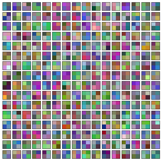
尽管我们没有训练网络到收敛,我们可以注意到不同的补丁显示出不同的模式。有些与其他相似,而有些则非常不同。这些可视化在较大图像大小时更为显著。
同样,我们可以可视化原始卷积核。这可以帮助我们理解给定卷积核的感受模式。
# 首先,打印出不是逐点卷积的卷积层的索引。
for i, layer in enumerate(conv_mixer_model.layers):
    if isinstance(layer, layers.DepthwiseConv2D):
        if layer.get_config()["kernel_size"] == (5, 5):
            print(i, layer)

idx = 26  # 取网络中间的一个卷积核。

kernel = conv_mixer_model.layers[idx].get_weights()[0]
kernel = np.expand_dims(kernel.squeeze(), axis=2)
visualization_plot(kernel)
5 <DepthwiseConv2D name=depthwise_conv2d, built=True>
12 <DepthwiseConv2D name=depthwise_conv2d_1, built=True>
19 <DepthwiseConv2D name=depthwise_conv2d_2, built=True>
26 <DepthwiseConv2D name=depthwise_conv2d_3, built=True>
33 <DepthwiseConv2D name=depthwise_conv2d_4, built=True>
40 <DepthwiseConv2D name=depthwise_conv2d_5, built=True>
47 <DepthwiseConv2D name=depthwise_conv2d_6, built=True>
54 <DepthwiseConv2D name=depthwise_conv2d_7, built=True>
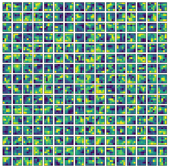
我们看到,卷积核中的不同滤波器具有不同的局部性范围,这种模式可能随着更多的训练而演变。
最后备注
最近有一个趋势是将卷积与其他数据无关的操作(如自注意力)融合。以下工作是沿着这一研究方向的:
- ConViT (d'Ascoli et al.)
- CCT (Hassani et al.)
- CoAtNet (Dai et al.)