使用 pandas 探索和可视化区域属性

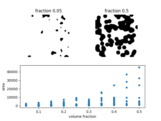
这个玩具示例展示了如何计算一系列10张图像中每个标记区域的大小。我们首先使用2D图像，然后使用3D图像。类似斑点的区域是合成生成的。随着体积分数（即斑点覆盖的像素或体素的比例）的增加，斑点（区域）的数量减少，单个区域的大小（面积或体积）可以变得越来越大。面积（大小）值以pandas兼容的格式提供，便于数据分析和可视化。

除了面积，还有许多其他区域属性可用。

import matplotlib.pyplot as plt
import numpy as np
import pandas as pd
import seaborn as sns

from skimage import data, measure


fractions = np.linspace(0.05, 0.5, 10)

2D 图像

images = [data.binary_blobs(volume_fraction=f) for f in fractions]

labeled_images = [measure.label(image) for image in images]

properties = ['label', 'area']

tables = [
    measure.regionprops_table(image, properties=properties) for image in labeled_images
]
tables = [pd.DataFrame(table) for table in tables]

for fraction, table in zip(fractions, tables):
    table['volume fraction'] = fraction

areas = pd.concat(tables, axis=0)

# Create custom grid of subplots
grid = plt.GridSpec(2, 2)
ax1 = plt.subplot(grid[0, 0])
ax2 = plt.subplot(grid[0, 1])
ax = plt.subplot(grid[1, :])
# Show image with lowest volume fraction
ax1.imshow(images[0], cmap='gray_r')
ax1.set_axis_off()
ax1.set_title(f'fraction {fractions[0]}')
# Show image with highest volume fraction
ax2.imshow(images[-1], cmap='gray_r')
ax2.set_axis_off()
ax2.set_title(f'fraction {fractions[-1]}')
# Plot area vs volume fraction
areas.plot(x='volume fraction', y='area', kind='scatter', ax=ax)
plt.show()

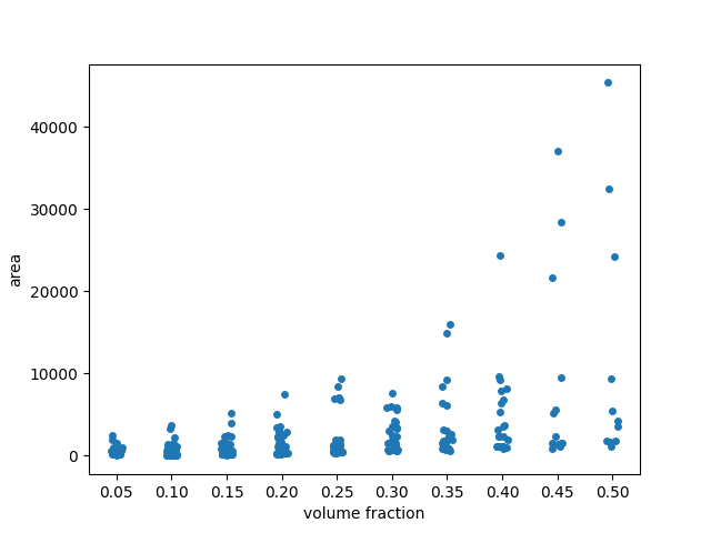
In the scatterplot, many points seem to be overlapping at low area values. To get a better sense of the distribution, we may want to add some ‘jitter’ to the visualization. To this end, we use seaborn.stripplot (from seaborn library for statistical data visualization) with argument jitter=True.

fig, ax = plt.subplots()
sns.stripplot(x='volume fraction', y='area', data=areas, jitter=True, ax=ax)
# Fix floating point rendering
ax.set_xticklabels([f'{frac:.2f}' for frac in fractions])
plt.show()

/Users/cw/baidu/code/fin_tool/github/scikit-image/doc/examples/segmentation/plot_regionprops_table.py:75: UserWarning:

set_ticklabels() should only be used with a fixed number of ticks, i.e. after set_ticks() or using a FixedLocator.

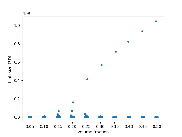
3D 图像

在三维中进行同样的分析，我们发现了一种更为戏剧性的行为：当体积分数超过约0.25时，团块会合并成一个巨大的单块。这对应于统计物理学和图论中的 渗透阈值。

images = [data.binary_blobs(length=128, n_dim=3, volume_fraction=f) for f in fractions]

labeled_images = [measure.label(image) for image in images]

properties = ['label', 'area']

tables = [
    measure.regionprops_table(image, properties=properties) for image in labeled_images
]
tables = [pd.DataFrame(table) for table in tables]

for fraction, table in zip(fractions, tables):
    table['volume fraction'] = fraction

blob_volumes = pd.concat(tables, axis=0)

fig, ax = plt.subplots()
sns.stripplot(x='volume fraction', y='area', data=blob_volumes, jitter=True, ax=ax)
ax.set_ylabel('blob size (3D)')
# Fix floating point rendering
ax.set_xticklabels([f'{frac:.2f}' for frac in fractions])
plt.show()

/Users/cw/baidu/code/fin_tool/github/scikit-image/doc/examples/segmentation/plot_regionprops_table.py:107: UserWarning:

set_ticklabels() should only be used with a fixed number of ticks, i.e. after set_ticks() or using a FixedLocator.