Note

Go to the end to download the full example code. or to run this example in your browser via Binder

scikit-learn 0.22 版本发布亮点#

我们很高兴地宣布发布 scikit-learn 0.22 版本，该版本包含许多错误修复和新功能！以下是本次发布的一些主要功能。有关所有更改的详尽列表，请参阅 release notes 。

要安装最新版本（使用 pip）:

pip install --upgrade scikit-learn

或使用 conda:

conda install -c conda-forge scikit-learn

新绘图 API#

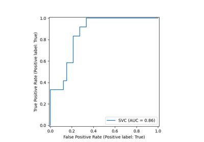
一个新的绘图API可用于创建可视化图表。这个新的API允许快速调整图表的视觉效果，而无需进行任何重新计算。还可以在同一个图中添加不同的图表。以下示例展示了 plot_roc_curve ，但也支持其他绘图工具，如 plot_partial_dependence 、 plot_precision_recall_curve 和 plot_confusion_matrix 。在:ref:用户指南 <visualizations> 中了解更多关于这个新API的信息。

import matplotlib.pyplot as plt

from sklearn.datasets import make_classification
from sklearn.ensemble import RandomForestClassifier

# from sklearn.metrics import plot_roc_curve
from sklearn.metrics import RocCurveDisplay
from sklearn.model_selection import train_test_split
from sklearn.svm import SVC

X, y = make_classification(random_state=0)
X_train, X_test, y_train, y_test = train_test_split(X, y, random_state=42)

svc = SVC(random_state=42)
svc.fit(X_train, y_train)
rfc = RandomForestClassifier(random_state=42)
rfc.fit(X_train, y_train)

# plot_roc_curve在1.2版本中已被移除。从1.2版本开始，请使用RocCurveDisplay。
# svc_disp = plot_roc_curve(svc, X_test, y_test)
# rfc_disp = plot_roc_curve(rfc, X_test, y_test, ax=svc_disp.ax_)
svc_disp = RocCurveDisplay.from_estimator(svc, X_test, y_test)
rfc_disp = RocCurveDisplay.from_estimator(rfc, X_test, y_test, ax=svc_disp.ax_)
rfc_disp.figure_.suptitle("ROC curve comparison")

plt.show()

堆叠分类器和回归器#

StackingClassifier 和 StackingRegressor 允许您使用最终分类器或回归器来堆叠估计器。堆叠泛化包括堆叠各个估计器的输出，并使用分类器计算最终预测。堆叠允许通过使用各个估计器的输出作为最终估计器的输入来利用每个估计器的优势。基础估计器在完整的 X 上进行拟合，而最终估计器使用基础估计器的交叉验证预测通过 cross_val_predict 进行训练。

请参阅用户指南了解更多信息。

from sklearn.datasets import load_iris
from sklearn.ensemble import StackingClassifier
from sklearn.linear_model import LogisticRegression
from sklearn.model_selection import train_test_split
from sklearn.pipeline import make_pipeline
from sklearn.preprocessing import StandardScaler
from sklearn.svm import LinearSVC

X, y = load_iris(return_X_y=True)
estimators = [
    ("rf", RandomForestClassifier(n_estimators=10, random_state=42)),
    ("svr", make_pipeline(StandardScaler(), LinearSVC(dual="auto", random_state=42))),
]
clf = StackingClassifier(estimators=estimators, final_estimator=LogisticRegression())
X_train, X_test, y_train, y_test = train_test_split(X, y, stratify=y, random_state=42)
clf.fit(X_train, y_train).score(X_test, y_test)

0.9473684210526315

基于排列的特征重要性#

:func:` inspection.permutation_importance`可以用于获取任何已拟合估计器的每个特征的重要性估计：

import matplotlib.pyplot as plt
import numpy as np

from sklearn.datasets import make_classification
from sklearn.ensemble import RandomForestClassifier
from sklearn.inspection import permutation_importance

X, y = make_classification(random_state=0, n_features=5, n_informative=3)
feature_names = np.array([f"x_{i}" for i in range(X.shape[1])])

rf = RandomForestClassifier(random_state=0).fit(X, y)
result = permutation_importance(rf, X, y, n_repeats=10, random_state=0, n_jobs=2)

fig, ax = plt.subplots()
sorted_idx = result.importances_mean.argsort()
ax.boxplot(
    result.importances[sorted_idx].T, vert=False, labels=feature_names[sorted_idx]
)
ax.set_title("Permutation Importance of each feature")
ax.set_ylabel("Features")
fig.tight_layout()
plt.show()

/app/scikit-learn-main-origin/examples/release_highlights/plot_release_highlights_0_22_0.py:100: MatplotlibDeprecationWarning:

The 'labels' parameter of boxplot() has been renamed 'tick_labels' since Matplotlib 3.9; support for the old name will be dropped in 3.11.

原生支持梯度提升中的缺失值#

ensemble.HistGradientBoostingClassifier 和 ensemble.HistGradientBoostingRegressor 现在原生支持缺失值（NaN）。这意味着在训练或预测时不需要进行数据插补。

from sklearn.ensemble import HistGradientBoostingClassifier

X = np.array([0, 1, 2, np.nan]).reshape(-1, 1)
y = [0, 0, 1, 1]

gbdt = HistGradientBoostingClassifier(min_samples_leaf=1).fit(X, y)
print(gbdt.predict(X))

[0 0 1 1]

预计算稀疏最近邻图#

大多数基于最近邻图的估计器现在接受预计算的稀疏图作为输入，以便在多个估计器拟合中重复使用相同的图。要在管道中使用此功能，可以使用 memory 参数以及两个新转换器之一，neighbors.KNeighborsTransformer 和 neighbors.RadiusNeighborsTransformer 。预计算也可以由自定义估计器执行，以使用替代实现，例如近似最近邻方法。更多详细信息请参见用户指南。

from tempfile import TemporaryDirectory

from sklearn.manifold import Isomap
from sklearn.neighbors import KNeighborsTransformer
from sklearn.pipeline import make_pipeline

X, y = make_classification(random_state=0)

with TemporaryDirectory(prefix="sklearn_cache_") as tmpdir:
    estimator = make_pipeline(
        KNeighborsTransformer(n_neighbors=10, mode="distance"),
        Isomap(n_neighbors=10, metric="precomputed"),
        memory=tmpdir,
    )
    estimator.fit(X)

    # 我们可以减少邻居的数量，并且图不会被重新计算。
    estimator.set_params(isomap__n_neighbors=5)
    estimator.fit(X)

KNN 基于插补#

我们现在支持使用 k-近邻算法完成缺失值的插补。

每个样本的缺失值使用在训练集中找到的 n_neighbors 个最近邻的平均值进行填补。如果两个样本在都不缺失的特征上接近，则认为它们是接近的。默认情况下，使用支持缺失值的欧几里得距离度量 nan_euclidean_distances 来找到最近邻。

树修剪#

现在可以在构建树之后修剪大多数基于树的估计器。修剪基于最小成本复杂度。详细信息请参阅:ref:用户指南 <minimal_cost_complexity_pruning> 。

X, y = make_classification(random_state=0)

rf = RandomForestClassifier(random_state=0, ccp_alpha=0).fit(X, y)
print(
    "Average number of nodes without pruning {:.1f}".format(
        np.mean([e.tree_.node_count for e in rf.estimators_])
    )
)

rf = RandomForestClassifier(random_state=0, ccp_alpha=0.05).fit(X, y)
print(
    "Average number of nodes with pruning {:.1f}".format(
        np.mean([e.tree_.node_count for e in rf.estimators_])
    )
)

Average number of nodes without pruning 22.3
Average number of nodes with pruning 6.4

从 OpenML 获取数据框#

datasets.fetch_openml 现在可以返回 pandas 数据框，从而正确处理异构数据集：

from sklearn.datasets import fetch_openml

titanic = fetch_openml("titanic", version=1, as_frame=True, parser="pandas")
print(titanic.data.head()[["pclass", "embarked"]])

   pclass embarked
     1        S
     1        S
     1        S
     1        S
     1        S

检查估计器的scikit-learn兼容性#

开发人员可以使用 check_estimator 检查其scikit-learn兼容估计器的兼容性。例如， check_estimator(LinearSVC()) 可以通过。

我们现在提供了一个特定于 pytest 的装饰器，它允许 pytest 独立运行所有检查并报告失败的检查。

..注意:: 此条目在版本 0.24 中略有更新，不再支持传递类：请传递实例。

from sklearn.linear_model import LogisticRegression
from sklearn.tree import DecisionTreeRegressor
from sklearn.utils.estimator_checks import parametrize_with_checks


@parametrize_with_checks([LogisticRegression(), DecisionTreeRegressor()])
def test_sklearn_compatible_estimator(estimator, check):
    check(estimator)

ROC AUC 现在支持多类分类#

roc_auc_score 函数现在也可以用于多类分类。目前支持两种平均策略：一对一算法计算成对 ROC AUC 分数的平均值，一对多算法计算每个类别相对于所有其他类别的 ROC AUC 分数的平均值。在这两种情况下，多类 ROC AUC 分数都是根据模型对样本属于特定类别的概率估计计算的。OvO 和 OvR 算法支持均匀加权（ average='macro' ）和按流行度加权（ average='weighted' ）。

请参阅用户指南了解更多信息。

from sklearn.datasets import make_classification
from sklearn.metrics import roc_auc_score
from sklearn.svm import SVC

X, y = make_classification(n_classes=4, n_informative=16)
clf = SVC(decision_function_shape="ovo", probability=True).fit(X, y)
print(roc_auc_score(y, clf.predict_proba(X), multi_class="ovo"))